Bayesian Optimization

Alexander Schoch,21/01/2025•programming python english machine learning algorithm

Bayesian Optimization is a method for finding the maximum value of an objective function that is unknown and costly to evaluate.

Example: We’d like to optimize a chemical reaction that produces a compound C. In order to maximize output, we need to find the temperature which the reaction produces the most amount of C at (i.e. has the largest yield). Thus, there is some function $Y(T)$ that correlates the yield with the reaction temperature, but we don’t know this function. We could just try to measure the reaction at different temperatures, but this would take a very long time, as running the reaction once (= sampling) takes, say, two days.

The goal of bayesian optimization is to find the maximum of a function (e.g. the temperature with maximum yield) by measuring the least sample points. More precisely, BO calculates the most probable maximum given a certain number of evaluations.

How does BO work?

Roughly, BO works by applying the following steps:

Initial samples

Before running the BO algorithm, we evaluate our function $N$ number of times, where $N$ can be any positive integer. At the start, we have no idea where the optimum might be, and what our objective function might look like, so it makes sense to start with an initial sampling.

Objective Function with three samples points already measured

Main Loop

Now, we repeat the following steps until either

our budget is used up (e.g. we have one month to measure all data points), or
the improvement from step to step is very small.

Surrogate Model

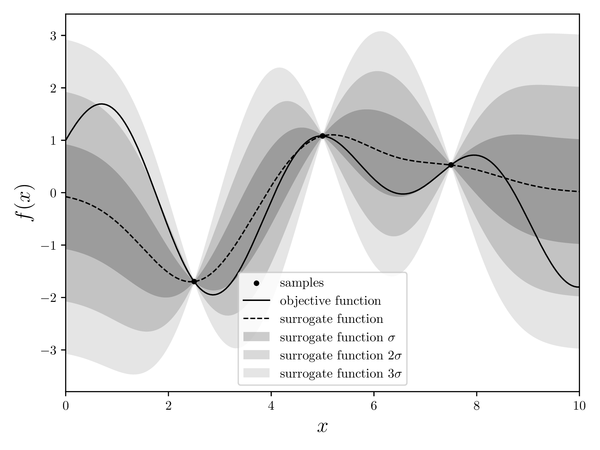
Through the points that we already measured, we fit a surrogate model. This model tries to estimate what the objective function might be, and assigns a standard deviation to each point. The surrogate model is very precise (low standard deviation) close to the points we measured. This makes sense: The points that are already known are “fixed”, so there is not much wiggle room in the proximity of these points.

There are many methods that can be used for this task, but most BO implementations use a Gaussian regression, also called “Kriging”.

Surrogate model with mean and standard deviation for three points

Acquisition Function

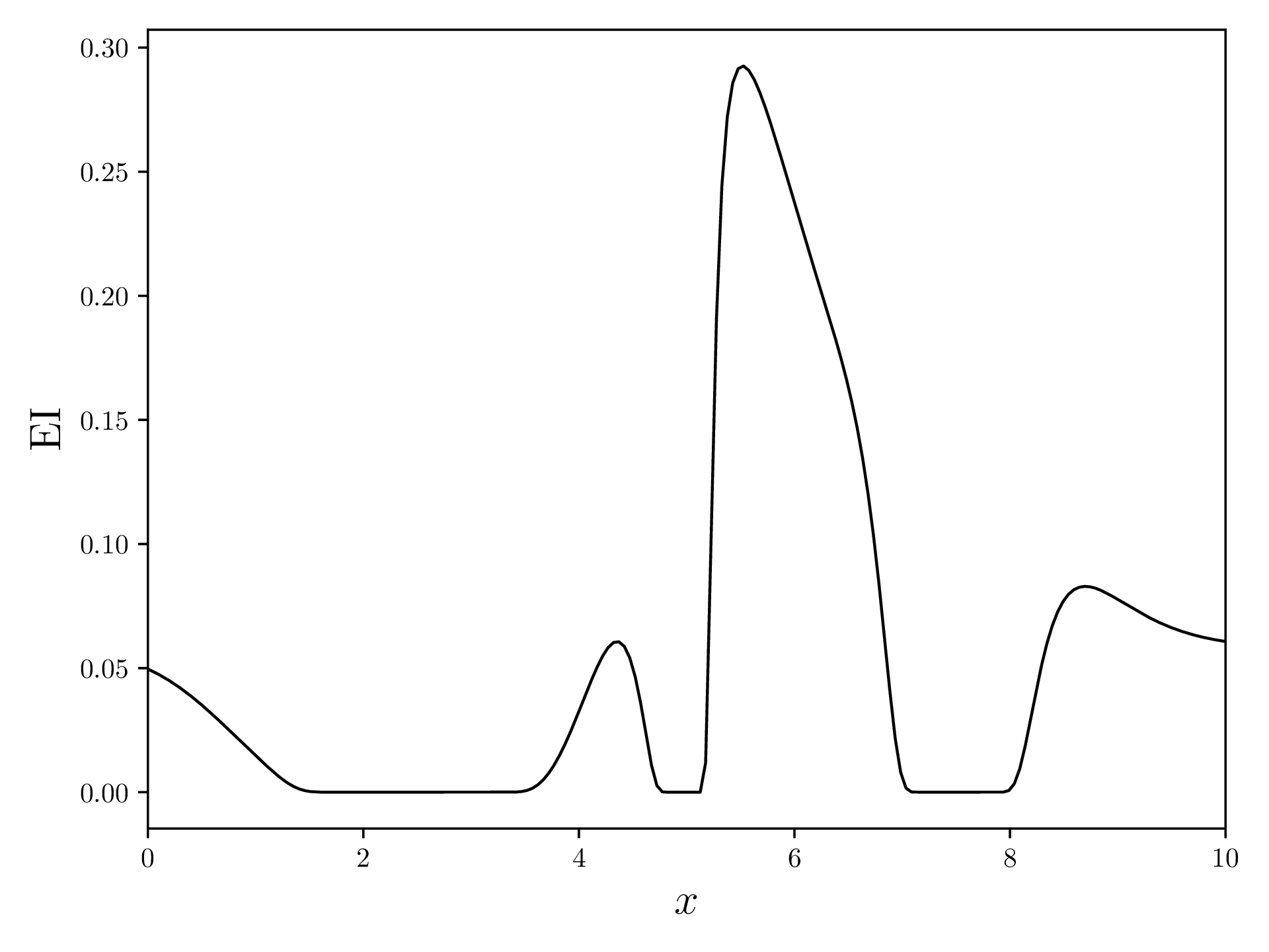
Next, we try to figure out where it makes the most sense to measure a new sample point. There are multiple AF that we can use, but one of the most commonly used ones is “Expected Improvement”. This AF caulcates, for each $x$ , the expected value for the improvement function for $f(x)$ .

The EI of the above example looks like this:

Expected Improvement of the above surrogate model

Measure a new Sample

The acquisition function now tells us where the best point for a new measurement lies. For this, we take the maximum of the acquisition function and use its $x$ value for a new evaluation of the objective function.

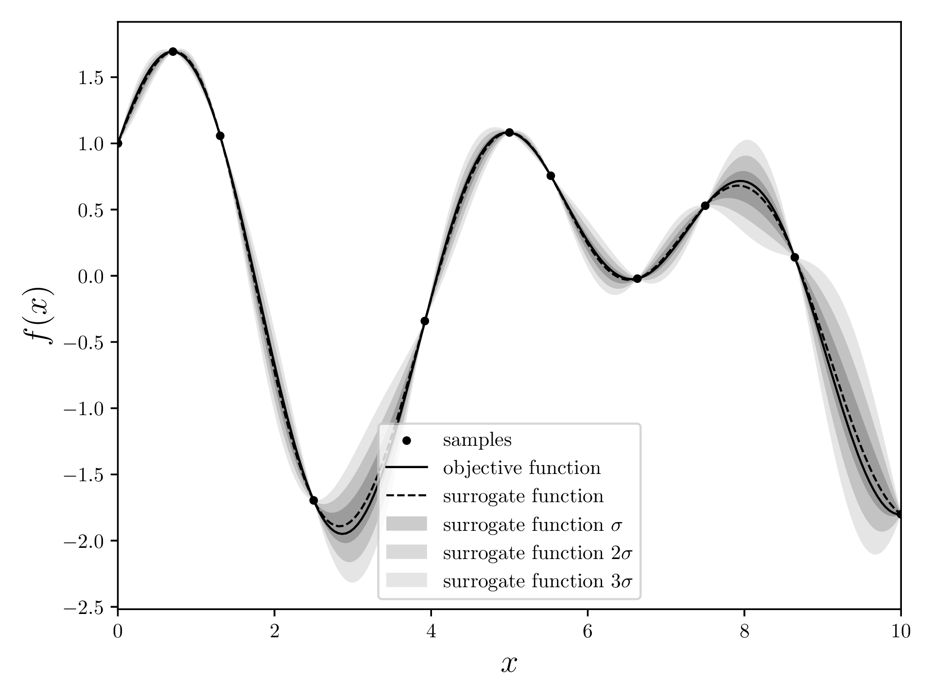
Result

After the main loop finishes, we caulcate the surrogate model once more and return the maximum of this model. This is the supposed global maximum of the objective function. In this case, the maximum is at $x^* = 0.704$ with a maximum of $f(x^*) = 1.693$ .

Let’s implement it!

First, create a new python venv, activate it and install all the necessary packages.


python -m venv venv
source venv/bin/activate # depends on the OS
 
pip install numpy scipy matplotlib

Let’s create a new python file and import all necessary libraries.


import os
import numpy as np
import matplotlib.pyplot as plt
 
from functools import reduce
from scipy.stats import norm

Next, let’s define a few constants that we can use later. DOMAIN is the extent of the $x$ axis, INITIAL_SAMPLES defines how many points we want to evaluate at the start, BUGDET is the number of iterations and machine_epsilon will be relevant later.


DOMAIN=[0,10]
INITIAL_SAMPLES=3
BUDGET=10
 
machine_epsilon = np.finfo(np.float32).eps

Objective Function

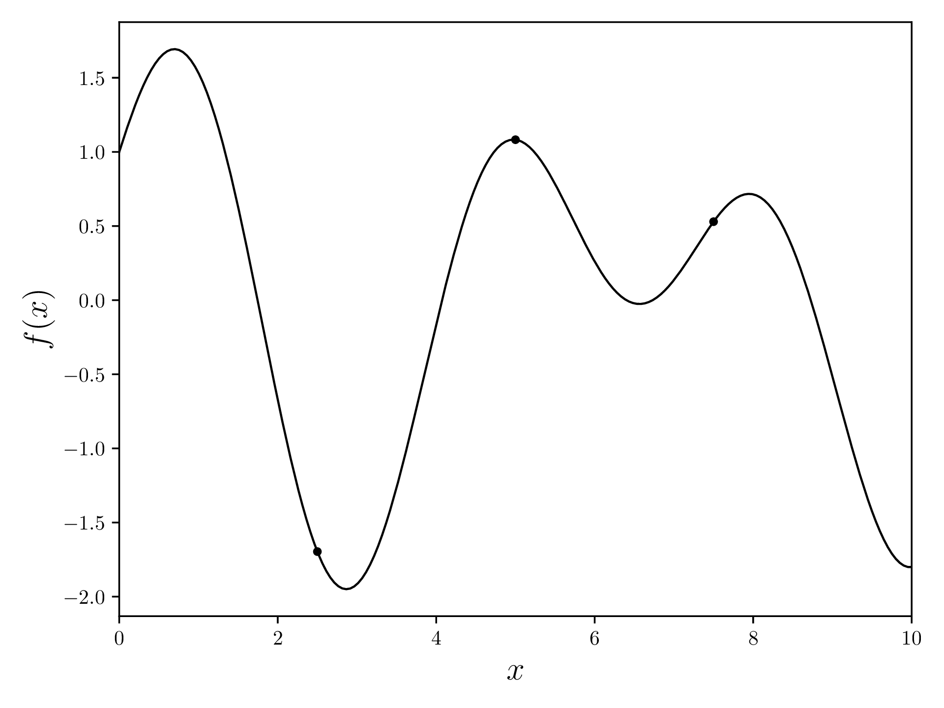
Alright, let’s define an objective function that our BO will try to optimize. For this example, I used

f(x) = \sin 1.7x + \cos x,

because it has a clear maximum and looks somewhat interesting.


objective_function = lambda x: np.sin(1.7 * x) + np.cos(x)

Now, we evaluate this function thrice at equidistant positions.


samples = np.array([[x, objective_function(x)] for x in np.linspace(*DOMAIN, INITIAL_SAMPLES+2)[1:-1]])


[[ 2.5        -1.69613297]
 [ 5.          1.0821493 ]
 [ 7.5         0.52923445]]

Plot the objective function together with the evaluated samples. As samples is an array of [x, y], we transpose (.T) and take the columns for plotting.


fig, ax = plt.subplots(figsize=(12.8, 4.8))
 
xvalues = np.linspace(*DOMAIN, 200)
yvalues = objective_function(xvalues)
 
ax.plot(xvalues, yvalues, linewidth=1, color='black')
ax.scatter(*samples.T, s=10, c='black')
ax.set_xlabel(r'$x$', fontsize=16)
ax.set_ylabel(r'$f(x)$', fontsize=16)
ax.set_xlim(*DOMAIN)
 
plt.tight_layout()
os.makedirs('output', exist_ok=True)
plt.savefig(os.path.join('output', 'objective_function.pdf'))
plt.close('all')

Surrogate Model (Gaussian Regression)

Covariance

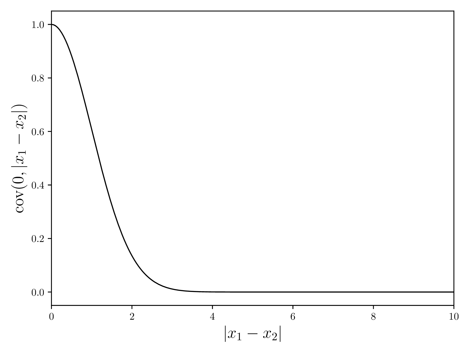
For the Gaussian Regression, we first need a covariance function. This function will, given two $x$ values $x_1$ and $x_2$ , return a value that describes how well these values correlate. For this demonstration, we use the Squared Exponential Kernel, which has a high correlation for values that are close and a low correlation for far apart values.

The Squared Exponential Kernel is defined as (source )

K(x_1, x_2) = \exp -\frac{1}{2}|x_1 - x_2|^2

and looks something like this:

Squared Exponential Kernel as a function of the distance between x1 and x2

In Python:


squaredExponentialKernel = lambda x1, x2: np.exp(-np.linalg.norm(x1 - x2)**2 / 2)

Now, we write a function that generates a covariance matrix given two input vectors $x_1$ and $x_2$ , as well as a kernel function. The covariance of an element with itself is the variance.


covariance = lambda x1, x2, kernel: np.array([[kernel(a, b) for b in x2] for a in x1])


In [2]: covariance([1, 2, 3], [1, 2, 3], squaredExponentialKernel)
Out[2]: 
array([[1.        , 0.60653066, 0.13533528],
       [0.60653066, 1.        , 0.60653066],
       [0.13533528, 0.60653066, 1.        ]])

Here, 1 and 3 are further apart, so their covariance is lower.

Gaussian Regression

The Gaussian Regression (as mean $\mu$ and covariance $\text{cov}$ ) is defined as (source )

\mu = K(X_*, X) \left( K(X, X) + I \right)^{-1} \mathbf{y}

and

\text{cov} = K(X_*, X_*) - K(X_*, X) \left( K(X, X) + I \right)^{-1} K(X, X_*)

with $X$ being the $x$ values of the samples, $\mathbf{y}$ the $y$ values of the samples and and $X_*$ the values at which we wish to calculate the Gaussian Regression.

We now write a function that implements these expressions. The machine_epsilon is the smallest value a float32 can store and prevents values from being 0 without actually disturbing the calculations. Some operations will throw an error if a value is 0.

After calculating $\mu$ and $\text{cov}$ , we calculate the standard deviation at each point by taking the diagonal elements (= variance) and returning the square root (= standard deviation).


def gaussian_regression(x, y, predict, kernel=squaredExponentialKernel):
    # K(X, X) + I
    K = covariance(x, x, kernel) + machine_epsilon * np.identity(len(x))
    # K(X_*, X)
    Ks = covariance(predict, x, kernel)
    # K(X*, X*)
    Kss = covariance(predict, predict, kernel)
 
    K_inv = np.linalg.inv(K)
 
    mean = np.dot(
        Ks,
        np.dot(
            K_inv,
            y
        )
    )
 
    cov = Kss - np.dot(
        Ks,
        np.dot(
            K_inv,
            Ks.T
        )
    )
 
    cov += machine_epsilon * np.ones(np.shape(cov)[0])
 
    std = np.sqrt(np.diag(cov))
 
    return mean, std

We can now use this function to calculate the surrogate model


mean, std = gaussian_regression(*samples.T, xvalues, kernel=squaredExponentialKernel)

and plot it. I plot three standard deviations here in order to visualize the diminishing probability of a measurement actually being there.


fig, ax = plt.subplots(figsize=(12.8, 4.8))
ax.scatter(*np.array(samples).transpose(), s=10, c='black', label=r'samples')
ax.plot(xvalues, objective_function(xvalues), color='black', linewidth=1, label='objective function')
ax.plot(xvalues, mean, linestyle='--', color='black', linewidth=1, label=r'surrogate function')
ax.fill_between(xvalues, mean + std, mean - std, alpha=0.2, color='black', label=r'surrogate function $\sigma$', linewidth=0)
ax.fill_between(xvalues, mean + 2*std, mean - 2*std, alpha=0.15, color='black', label=r'surrogate function $2\sigma$', linewidth=0)
ax.fill_between(xvalues, mean + 3*std, mean - 3*std, alpha=0.1, color='black', label=r'surrogate function $3\sigma$', linewidth=0)
 
ax.set_xlim(*DOMAIN)
ax.set_xlabel(r'$x$', fontsize=16)
ax.set_ylabel(r'$f(x)$', fontsize=16)
 
ax.legend()
plt.tight_layout()
plt.savefig(os.path.join('output', f'gaussian_regression.pdf'))
plt.close('all')

Acquisition Function

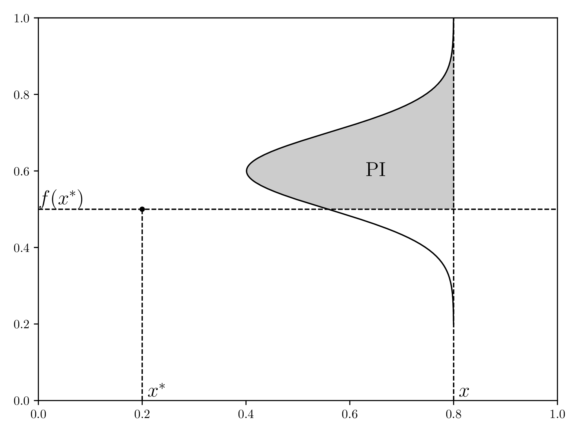
In order to understand Expected Improvement, let’s look at “Probability of Improvement”, PI, first.

For a given current best value in our samples ( $x^*$ and $f(x^*)$ ), PI defines a function $I(x)$ that is the probability that a new point measured at this $x$ will result in a better best value. For this, the surrogate model from step 1 defines a normal distribution in the $y$ direction for each $x$ , which is shown by how wide the gray area is at a position $x$ .

Visualization of PI, redrawn from here :

EI will now not only consider if a certain measurement will improve the current best, but also by how much.

For implementing EI, we first need to know the best point we currently have. This can be done using the reduce function:


best_point = reduce(lambda point, m: point if point[1] > m[1] else m, samples)

reduce is a function commonly used in functional programming and reduces list down to a single value. It does this by taking a function that takes a value and an accumulator and returns the new accumulator.

EI is defined as (source )

\text{EI}(x; \xi) = \delta \Phi\left(\frac{\delta}{\sigma}\right) + \sigma\varphi\left(\frac{\delta}{\sigma}\right)

with $\delta = \mu - f(x^*) - \xi$ , $\varphi$ being the probability density function of the normal distribution (scipy.stats.norm.pdf) and $\Phi$ being the cumulative density function for the normal distribution (scipy.stats.norm.cdf).

The $\xi$ value controls “exploration” vs. “exploitation”: If $\xi$ is close to zero, BO will often try to find local optima and thus converge quicker, with the risk of a local optimum not being the global optimum. For large $\xi$ , BO will “jump around” more and thus potentially evaluate points at places that are further away from the previous point.

To write this, we first define an empty list EI and then loop over all points to calculate $\text{EI}(x)$ . Note that scipy.stats.norm is a class that we have to instanciate with the correct standard deviation first.


xi = 0.1
 
EI = []
for i in range(len(xvalues)):
    delta = mean[i] - best_point[1] - xi
    std[std == 0] = np.inf
    z = delta / std[i]
    unit_norm = norm(scale=std[i])
    EI.append(delta * unit_norm.cdf(z) + std[i] * unit_norm.pdf(z))

Now, we can plot EI:


fig, ax = plt.subplots(figsize=(12.8, 4.8))
ax.plot(xvalues, EI, linewidth=1, color='black')
 
ax.set_xlim(*DOMAIN)
ax.set_xlabel(r'$x$', fontsize=16)
ax.set_ylabel(r'$\text{EI}$', fontsize=16)
 
plt.tight_layout()
plt.savefig(os.path.join('output', f'expected_improvement.pdf'))
plt.close('all')

Measure a new Sample

Last, we find the maximum in EI and use this $x$ value to measure a new sample from the objective function. We append this new [x, y] pair to the samples array.


max_EI_index = np.argmax(EI)
max_EI = EI[max_EI_index]
 
samples = np.array([*samples, [xvalues[max_EI_index], objective_function(xvalues[max_EI_index])]])

Return Maximum

The steps Surrogate Model, Acquisition Function and Measure a new Sample are now repeated BUDGET times.

After that, generate the surrogate model once more and find the maximum thereof.


mean, std = gaussian_regression(*samples.T, xvalues, kernel=squaredExponentialKernel)
max_index = np.argmax(mean)
 
print(f"Maximum found at {[xvalues[max_index], mean[max_index]]}")

Full Code

The steps in the loop are here put into a loop and each iteration’s plots are saved using the loop iterator. The zero_pad function just makes sure that each iterator has the same number of digits (e.g. 0024), which allows for correct sorting by your OS.


import os
import numpy as np
import matplotlib.pyplot as plt
 
from functools import reduce
from scipy.stats import norm
 
DOMAIN=[0,10]
INITIAL_SAMPLES=3
BUDGET=10
 
machine_epsilon = np.finfo(np.float32).eps
 
objective_function = lambda x: np.sin(1.7 * x) + np.cos(x)
samples = np.array([[x, objective_function(x)] for x in np.linspace(*DOMAIN, INITIAL_SAMPLES+2)[1:-1]])
 
 
# --- Objective Function ---
fig, ax = plt.subplots(figsize=(12.8, 4.8))
 
xvalues = np.linspace(*DOMAIN, 200)
yvalues = objective_function(xvalues)
 
ax.plot(xvalues, yvalues, linewidth=1, color='black')
ax.scatter(*samples.T, s=10, c='black')
ax.set_xlabel(r'$x$', fontsize=16)
ax.set_ylabel(r'$f(x)$', fontsize=16)
ax.set_xlim(*DOMAIN)
 
plt.tight_layout()
os.makedirs('output', exist_ok=True)
plt.savefig(os.path.join('output', 'objective_function.pdf'))
plt.close('all')
 
 
# --- Covariance ---
squaredExponentialKernel = lambda x1, x2: np.exp(-np.linalg.norm(x1 - x2)**2 / 2)
covariance = lambda x1, x2, kernel: np.array([[kernel(a, b) for b in x2] for a in x1])
 
yvalues = [squaredExponentialKernel(0, x) for x in xvalues]
 
plt.plot(xvalues, yvalues, color='black', linewidth=1)
 
plt.xlim(*DOMAIN)
plt.xlabel(r'$|x_1 - x_2|$', fontsize=16)
plt.ylabel(r'$\text{cov}(0, |x_1 - x_2|)$', fontsize=16)
 
plt.tight_layout()
plt.savefig(os.path.join('output', 'squaredExponentialKernel.pdf'))
plt.close('all')
 
 
# --- Gaussian Regression ---
def gaussian_regression(x, y, predict, kernel=squaredExponentialKernel):
    K = covariance(x, x, kernel) + machine_epsilon * np.identity(len(x))
    Ks = covariance(predict, x, kernel)
    Kss = covariance(predict, predict, kernel)
 
    K_inv = np.linalg.inv(K)
 
    mean = np.dot(
        Ks,
        np.dot(
            K_inv,
            y
        )
    )
 
    cov = Kss - np.dot(
        Ks,
        np.dot(
            K_inv,
            Ks.T
        )
    )
 
    cov += machine_epsilon * np.ones(np.shape(cov)[0])
 
    std = np.sqrt(np.diag(cov))
 
    return mean, std
 
def zero_pad(value, max_number):
    num_digits = int(np.log10(max_number-1)) + 1
    return str(value).zfill(num_digits)
 
for i in range(BUDGET):
    print(f"==> Iteration {i+1}/{BUDGET}")
    filename_suffix = zero_pad(i, BUDGET)
 
 
    # --- Surrogate Model ---
    mean, std = gaussian_regression(*samples.T, xvalues, kernel=squaredExponentialKernel)
 
    fig, ax = plt.subplots(figsize=(12.8, 4.8))
    ax.scatter(*np.array(samples).transpose(), s=10, c='black', label=r'samples')
    ax.plot(xvalues, objective_function(xvalues), color='black', linewidth=1, label='objective function')
    ax.plot(xvalues, mean, linestyle='--', color='black', linewidth=1, label=r'surrogate function')
    ax.fill_between(xvalues, mean + std, mean - std, alpha=0.2, color='black', label=r'surrogate function $\sigma$', linewidth=0)
    ax.fill_between(xvalues, mean + 2*std, mean - 2*std, alpha=0.15, color='black', label=r'surrogate function $2\sigma$', linewidth=0)
    ax.fill_between(xvalues, mean + 3*std, mean - 3*std, alpha=0.1, color='black', label=r'surrogate function $3\sigma$', linewidth=0)
 
    ax.set_xlim(*DOMAIN)
    ax.set_xlabel(r'$x$', fontsize=16)
    ax.set_ylabel(r'$f(x)$', fontsize=16)
 
    ax.legend()
    plt.tight_layout()
    plt.savefig(os.path.join('output', f'gaussian_regression_{filename_suffix}.pdf'))
    plt.close('all')
 
 
    # --- Acquisition Function ---
    best_point = reduce(lambda point, m: point if point[1] > m[1] else m, samples)
    xi = 0.1
 
    EI = []
    for i in range(len(xvalues)):
        delta = mean[i] - best_point[1] - xi
        std[std == 0] = np.inf
        z = delta / std[i]
        unit_norm = norm(scale=std[i])
        EI.append(delta * unit_norm.cdf(z) + std[i] * unit_norm.pdf(z))
 
    fig, ax = plt.subplots(figsize=(12.8, 4.8))
    ax.plot(xvalues, EI, linewidth=1, color='black')
 
    ax.set_xlim(*DOMAIN)
    ax.set_xlabel(r'$x$', fontsize=16)
    ax.set_ylabel(r'$\text{EI}$', fontsize=16)
 
    plt.tight_layout()
    plt.savefig(os.path.join('output', f'expected_improvement_{filename_suffix}.pdf'))
    plt.close('all')
 
    # --- measure another sample ---
    max_EI_index = np.argmax(EI)
    max_EI = EI[max_EI_index]
 
    samples = np.array([*samples, [xvalues[max_EI_index], objective_function(xvalues[max_EI_index])]])
 
 
# --- get maximum of surrogate model ---
mean, std = gaussian_regression(*samples.T, xvalues, kernel=squaredExponentialKernel)
max_index = np.argmax(mean)
 
print(f"Maximum found at {[xvalues[max_index], mean[max_index]]}")

Comments

Source Code

Subscribe via RSS.